Formula of the sum in figures

How do you create a sum of hour, minute column and multiple by a dollars an hour?

For example,.

10 h in the B1:B22 column

$30 / h in C1

Hi rp,.

"The hours and minutes" are lasting and if multiplied by a number, will be a result that is also a duration. So the first step is to convert this length to a number that represents the hours (and part of an hour), then multiply this number by a second number that represents the rate of pay in the number of Dollars (and fraction of a Dollar) per hour.

C2: = DUR2HOURS (B) * C$ 1

D2: = DUR2HOURS (B) * D$ 1

The values in the column of the hours are times.

Values in C1 and D1 are numbers.

Results in columns C and D are numbers, with the format of the cell value Currency with two decimal places.

Table built in numbers (Numbers ' 09) v2.3. The formulas are the same in numbers v3.

Kind regards

Barry

Tags: iWork

Similar Questions

Error number according to the sum


$88.00	$0.00	$88.00	$0.00
$275.00	$275.00	$0.00	$0.00
$275.00	$275.00	$0.00	$0.00
$275.00	$275.00	$0.00	$0.00
$275.00	$275.00	$0.00	$0.00
$275.00	$275.00	$0.00	$0.00
$275.00	$275.00	$0.00	$0.00
$275.00	$275.00	$0.00	$0.00
$275.00	$275.00	$0.00	$0.00
$275.00	$275.00	$0.00	$0.00
$275.00	$275.00	$0.00	$0.00
$275.00	$275.00	$0.00	$0.00
$275.00	$275.00	$0.00	$0.00
$85.70	$0.00	$85.70	$0.00
$275.00	$275.00	$0.00	$0.00
$275.00	$275.00	$0.00	$0.00
$275.00	$275.00	$0.00	$0.00
$275.00	$275.00	$0.00	$0.00
$275.00	$275.00	$0.00	$0.00
$275.00	$275.00	$0.00	$0.00
$275.00	$275.00	$0.00	$0.00
$275.00	$275.00	$0.00	$0.00
$275.00	$275.00	$0.00	$0.00
$275.00	$275.00	$0.00	$0.00
$525.00	$525.00	$0.00	$0.00
$275.00	$275.00	$0.00	$0.00
$375.00	$375.00	$0.00	$0.00
$410.00	$325.00	$85.00	$0.00
$550.00	$550.00	$0.00	$0.00
$275.00	$275.00	$0.00	$0.00
$300.00	$300.00	$0.00	$0.00
$275.00	$275.00	$0.00	$0.00
$275.00	$275.00	$0.00	$0.00
$400.00	$400.00	$0.00	$0.00
$420.00	$420.00	$0.00	$0.00
$275.00	$275.00	$0.00	$0.00
$275.00	$275.00	$0.00	$0.00
$280.00	$280.00	$0.00	$0.00
$275.00	$275.00	$0.00	$0.00
$275.00	$275.00	$0.00	$0.00
$400.00	$400.00	$0.00	$0.00
$275.00	$275.00	$0.00	$0.00
$355,00	$275.00	$80.00	$0.00
$275.00

$275.00

$0.00

$300.00

$0.00

$275.00

$0.00

$300.00

$0.00

$300.00

$0.00

$275.00

$0.00

$275.00

$0.00

$275.00

$0.00

$275.00

$0.00

$275.00

$0.00

$275.00

$0.00

$275.00

$0.00

$550.00

$0.00

$300.00

$0.00

$550.00

$0.00

$93.00

$0.00

$93.00

$0.00

$550.00

$0.00

$550.00

$0.00

$275.00

$0.00

$275.00

$0.00

$275.00

$0.00

$550.00

$0.00

$50.00

$0.00

$500.00

$0.00

$550.00

$0.00

$300.00

$215,40

$84,60

$0.00

$500.00

$0.00

$500.00

$0.00

$550.00

$0.00

$550.00

$0.00

$240.00

$145.00

$95.00

$0.00

$550.00

$0.00

$550.00

$0.00

$450.00

$0.00

$280.00

$0.00

$500.00

$0.00

$275.00

$0.00

$280.00

$0.00

$270.00

$0.00

$275.00

$0.00

$300.00

$0.00

$250.00

$0.00

$275.00

$0.00

$275.00

$0.00

$375.00

$275.00

$100.00

$0.00

$300.00

$0.00

$250.00

$0.00

$275.00

$0.00

$275.00

$0.00

$275.00

$0.00

$275.00

$0.00

$275.00

$0.00

$550.00

$0.00

$550.00

$0.00

$112.00

$0.00

$112.00

$0.00

$550.00

$0.00

$550.00

$0.00

$550.00

$0.00

$550.00

$0.00

$550.00

$0.00

$108.00

$0.00

$108.00

$0.00

$550.00

$0.00

$550.00

$0.00

$550.00

$0.00

$550.00

$0.00

$550.00

$0.00

$550.00

$0.00

$550.00

$0.00

$550.00

$0.00

$550.00

$0.00

$102,00

$0.00

$102,00

$0.00

$550.00

$0.00

$550.00

$0.00

$134.00

$0.00

$134.00

$0.00

$200.00

$0.00

$350.00

$0.00

$550.00

$0.00

$550.00

$0.00

$550.00

$0.00

$100.00

$0.00

$450.00

$0.00

$550.00

$0.00

$44282,70

$42565,40

$1167,30

$550.00

I the sum vertically downwards, but when I do my check is not. I guess to get $0 corresponding to the sum of $550.

Hi Henry,.

What is the formula in the cell with the Red 550? (Copy and paste in the document, please, not transcribed by hand).

What, in the line number of the line that is the last to contain this set of values: $100.00 $100.00, $0.00, $0.00?

Respect,

Barry

Returns the sum of the values of certain months

Hello

I have a table that I keep a record of my overtime. See below.

I want to do another table of the month (Jan, Feb, Mar etc.) and next to it the sum of all overtime worked each month.

My salary is developed from the 4th of each month to the 4th on the other, I am able to add up the values of the different months and specify between the 4th one on the 4th of another?

Thanks in advance.

One way to do would be to use SUMIFS.

The formula in B2, filled to the bottom:

= SUMIFS(Table 1::$E,Table 1::$A,">"&C2,Table 1::$A,"<"&D2)

The formula in C2, filled to the bottom:

= A2 + 4

The formula in D2, filled to the bottom:

= EOMONTH(A2,0) + 5

Column A contains strings of date and time in the format to display the month only.

SG

How the SUM cells including the text and the number?

Hello world

Someone can tell me how the SUM cells include the text and the number?

1 Bob 20

2 30 Jane

3 50 Jame

Total 100

Thank you

Hi Jordan,.

If the numbers are not always two digits, FIND the position of the space between the number and name:

Formula in B2 (fill down)

= FIND("",A2)

Then use the LEFT function to get the number in the column C:

Formula in C2 (fill down)

= LEFT (A2, B2)

This will give a text string (Tip: left-aligned).

Convert to a numeric value in the D column with the VALUE function:

Formula in D2 (fill down)

VALUE = (C2)

(Tip: propped right)

Table 1 has a header row and footer of the line, and the SUM is easy. Formula to the D8 footer line:

= SUM (D)

Kind regards

Ian.

Edit: You can hide columns B and C

Ian.

formulas in the menu drop-down?

Hello everyone, so the experience I've had here the last time it was amazing so why not come back to the question.

I have a spreadsheet that will be followed by my money in and out of the clinic. I want to create a drop down menu that will allow me to choose what percentage of compensation is due to a technician/doctor

Ex: if I want to that they get paid 40% I want G1 look something like this x.40 of the sum (B1) or if I want to give them a cost share & pay sum (B1)-(C1) - x.40 (F1)

Is it possible to make formulas in a pop-up menu? Thanks for any help you guys can provide on this...

Marshall

.

Do not run formula until the full input cells

Hello ladies and gentlemen

I'm not a user of regular broadcast sheet, there must be a good few years since I changed the numbers you use...

But I plug just your new car and I wanted a spreadsheet for just about track mileage and fuel MPG etc.

Self created one and it works very well in my goals.

I copied the formulas in cells, but the lines that have not been provided for future end of refuelling upward with being supplemented with nonsense

How can I avoid the form "in cell formulas' filling the cells up to that there are entries in the column of the figure of supply?

Perhaps easier if I show a picture

Yellow cells I get my numbers

Green cells contain formulas.

How can I stop the numbers filling in the Green columns until I enter numbers in the yellow?

As you see, the-9800 the ones and zeros of formula errors

I did some research... but no idea what word I'm looking for able to conduct a successful search. Tried such research than the job title and multiple similar on the same theme... but all from a blank test.

Here is the worksheet that I created:

http://paisnel.co.UK/upload/KIA.numbers

Thank you

Hi Neil,

This approach is to test your yellow column to see if it has a value. Len() will be taken into account the characters in a cell.

C3 = IF (LEN (B3) "> 0, B3−B2," "")

This formula will test a B3 value and if there is one subtract it from B2. If there is no value it returns "" which resembles a cell empty.

If B is always going to be a numeric value, you could simplify the test:

IF(B3>0,B3-B2,"")

Quinn

How to insert as an entry within the formula variable, the total time on the scope window?

How to insert, as an entry within the formula variable, the window of total time on the scope (i.e. of 20ms/div x 10 div = 200ms)?

HERE'S A SAMPLE QUESTION:

FORMULA FOR INTEGRAL ACTION:

STATISTICS:

Input variable: DPO4034 (CH1);

Box: number of samples.

FORMULA

Input variable 0: DPO4034 (CH1); alias: x 0

Input variable 1: 'time window Total out of scope?. " alias: x 1

Input variable 2: number of samples (CH1); alias: x 2

Under the operation Configuration: formula

Y = (x 0 ^ 2) *(x1/x2)

Output: Data 1 (CH1)

THEN, WITH THE HELP OF STATISTICS:

Input signal: data processing 1 (CH1)

Checkbox: SUM

Output: CH1 integral Action [has ^ 2s].

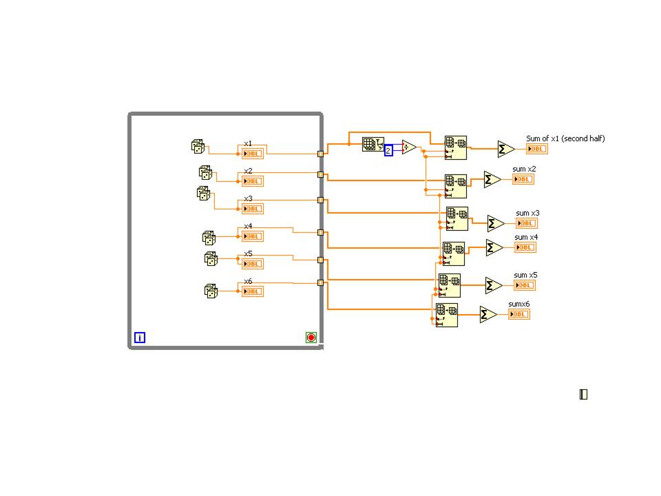
How take the sum of middle iteration last iteration?

Hello! PLS, can anyone help, I have six variables and you want to take the sum of each of the variables separately from the middle of the iteration to the last iteration (i.e. iteration 6 iteration 12). Attached are the vi file and data entry.

I won't mess with your design of control thingy... but here is the simple and direct way to the sum of the average in last interation. I use random numbers here, but you can enter your own values once you get out your straigthend formula.

Basically, it works like this: feed values into a tunnel of indexation. Which will make each set of values in an array whose length N where N is the number of iterations.

Find the array size and divide by 2. Remember that arrays start at index zero, so 12 iterations will give you 0,1,2,3,4,5,6,7,8,9,10,11.

You want the second half, so it's 6,7,8,9,10 and 11. Subset of the table to select 6 elements, starting with element 6... Then take the sum of table.

Formula member to sum based on a model

Hello
I have a question by creating a formula for a sum based on a model member.
In a cube, OSI, we have 2 sparse dimensions, which contains a hierarchy of alternative with shared members. There is a hierarchy of high maintenance new shared members are added each month.
I would like to remove this successor to the shared members hierarchy and replace it with a formula of Member. This hierarchy looks like this
Entity CC01 Summation
CC-01-100
CC-01-101
CC-01-111
etc.
I tried to add a member formula that corresponds to this model @MATCH ('Entity', ' CC-01 * ") and summarizes all CC - 01 *. My formula looks like this @SUM (@MATCH ('Entity', ' CC-01 * ")). It does not work. She added a few other totals which I have not yet studied.
Any idea is appreciated...
Thank you.

Hello

It is not necessary to take the name of the dimension of the mbrname. @MATCH (mbrName | genName | levName, 'boss')

Take the parent where the search should begin here. So, without other hierarchies.

It should work.

Kind regards

Philip Hulsebosch

Beginner problems - how to make the sum of the lists in a drop-down table

Hello
Please forgive my newness but I'm creating a table with 10 + lines and columns and need to calculate the sum of the columns. The user must select a number from a drop-down list and I would like to summarize these nbumbers at the bottom of the column, seems simple enough...
I have named each cell in the links tab but can't seem to find the script of the sum on the right. I just started using livecycle and have had a good experience so far.
I wish it was like excel where you just need to click or highlight the cells you want to summarize and do with it but I can't seem to find the easy button...
You can not simply highlight a column, name it and then use that name in a script to sum?
Thanks a lot for all the help and I have looked around, but can't get a grip on this one, so I apologize if this is requested before.
Go easy on me.

You have to be very accurate with referencing the fields or the formulas will not work. If you have renamed the fields of their default values, then you should reference them as you named the.

Here's an example of my hierarchy, called as you explained:

In this case, the use of scripts on the Total field will look like this:

this.rawValue = (Row1.A1.rawValue * 1) + (Row2.B1.rawValue * 1) + (Row3.C1.rawValue * 1) + (Row4.D1.rawValue * 1);

So that when I switch to preview, it behaves correctly:

CALCULATE the sum of the amounts?

Hey guys!

This script:

CLEAR      COMPUTES 
CLEAR     BREAKS

SET     feedback     off
SET     pagesize     5000
SET     linesize     50
SET     echo          off
SET     heading          on
SET     verify          off

COLUMN     User format     A8
COLUMN     Files format     999999999
COLUMN     Docs format     999999999
COLUMN     Pages format     999999999

COMPUTE SUM LABEL TOTAL OF "FILES", "DOCS", "PAGES"

PROMPT     ************************************************** 
PROMPT     *         Monthly File Activity by User          *
PROMPT     ************************************************** 
PROMPT      
PROMPT      
ACCEPT     StartDate     DATE FORMAT 'MMYYYY'      PROMPT 'Enter the month and year (MMYYYY): '
PROMPT     
PROMPT      List of users:
PROMPT      One
PROMPT      Two
PROMPT      Three
PROMPT      Four
PROMPT      Five
PROMPT      Six
PROMPT      Seven
PROMPT     UNKNOWN
PROMPT       
PROMPT     Type 'ALL', or leave blank, to select all users.
PROMPT      
ACCEPT     UserChoice     DEFAULT 'ALL'     PROMPT 'Please enter a user: '


SELECT
     (CREATOR_ID
                   WHEN     '1'     THEN     'One'
                 WHEN     '2'     THEN     'Two'
          WHEN     '3'     THEN     'Three'
          WHEN     '4'     THEN     'Four'
          WHEN     '5'     THEN     'Five'
          WHEN     '6'     THEN     'Six'
          WHEN     '7'     THEN     'Seven'
          ELSE     'UNKNOWN'
          END)     "USER",
     count       (distinct(substr(DOC_NAME,1,9))) AS Files,
     count     (DOC_IMAGE) AS Docs,
     sum     (DOC_PAGE) AS Pages
FROM
     TABLE1,
     TABLE2
WHERE
     DOC_DATE to_date('&StartDate','MMYYYY') AND last_day(to_date('&StartDate','MMYYYY'))
AND
     CREATOR_ID not in ('Thing','8','9')
AND
     ((CREATOR_ID
                   WHEN     '1'     THEN     'One'
                 WHEN     '2'     THEN     'Two'
          WHEN     '3'     THEN     'Three'
          WHEN     '4'     THEN     'Four'
          WHEN     '5'     THEN     'Five'
          WHEN     '6'     THEN     'Six'
          WHEN     '7'     THEN     'Seven'
          ELSE     'UNKNOWN'
          END) = UPPER('&UserChoice')
     OR
     '&UserChoice' = 'ALL')
GROUP BY
     CREATOR_ID
/

produces this result:

USER          FILES       DOCS      PAGES
-------- ---------- ---------- ----------
One             261       4276      18124
Two             364       5954      26913
Three           109       1996       8243
Four            178       3635      14554
Five            104       2657      11662
Six             308       6639      27887

I would like for a labeled sum TOTAL at the bottom of these figures. I thought that COMPUTE would take care of this, but it's not. Am I missing something? It will not add these to the top because they are already money from specific users? Insight? I'm new to SQL and would like to be pointed in the right direction. Thanks for your expertise!

I'm on a 10g system.

Calculation is not SQL and SQL * more.
The general syntax is
calculate the sum of... the * | * report

followed by
break the report
When this is necessary.

-----------
Sybrand Bakker
Senior Oracle DBA

How can I use the SUM function to calculate the number of employees in the comp. & deptnt?

I have two tables: employees and their departments. I'm figuring the total employees by the Department and the total employees of the entire society. I know I have to use the SUM function, but I can only calculate total employees by Department and company separately. I need to get this result:

DEPT_NAME     DEPT_TOTAL_SALARY         COMPANY_TOTAL_SALARY
RESEARCH                  10875                        29025
SALES                      9400                        29025    
ACCOUNTING                 8750                        29025      


This is my code:

SELECT department_name, SUM(salary) as total_salary
FROM employee, department
WHERE employee.department_id = department.department_id
GROUP BY department_name;

SELECT SUM(salary)
FROM employee;






Can somebody help please?
Thank you in advance.

Published by: user13675672 on January 30, 2011 14:29

Published by: user13675672 on January 30, 2011 14:31

Hello

Something like:

SELECT dname,
       dept_tot_sal,
       SUM (dept_tot_sal) OVER () comp_tot_sal
FROM   (SELECT   dname,
                 SUM (sal) dept_tot_sal
        FROM     dept, emp
        WHERE    dept.deptno = emp.deptno
        GROUP BY dname);

There might be a smarter way, with no re - select.

Concerning
Peter

Analytical functions:
http://download.Oracle.com/docs/CD/E11882_01/server.112/e17118/functions004.htm

How to find the sum of an element of the record multi block?
Hello

Hi I have form have a multi block record and sing record block. Multi block record for an element, namely Excise_value. I want to find the sum of total Excise_Value of the entire tape. How to get there.

Please guide me in this regard.

PS: I want to use the Formula property / summary forms

Thank you

Iqbal
For your unique record block, set the property of simple recording/precalculate summaries on YES.
And in BlockA, set the property of all the query to YES.

-Clément

Formula in the primary account not to ASO dimension hierarchy
Is this in any way by which I can write a formula in a primary account not dimension hierarchy. I have tagged this member as allowing multiple hierarchies and I can't adjust primary hierarchy as dynamic to ASO. so I put it as stored and now I want to write a formula for one of the members. I'm not able to put the formula for stored dimension.

is there a workaround or can you please suggest me something that might work

Thank you
You can have formulas in the dimensions (or hierarchies) marked as dynamic. If you have a dynamic hierarchy, you might substitute in there running sums.

Formula in the answers page
Hello!, I have a problem to make a table in the page of answers: I explain my problem with an example.

Suppose you have two dimensions and a measure

This two dimension have childs (A, B, C) (some dimensions are IDENTICAL).

Dimension1:
-A
B
-C

Dimension2:
-A
B
D

OK... now if I chose my measurement have a table like this:

Dim1 - Dim2 - measure
A-------------A------------10
---------------B------------15
---------------D------------12
B-------------A------------20
---------------B------------16
C-------------B------------20
---------------D-------------9

I would like two additional measures when Dim1 = Dim2 it shows date2 and what Dim1, Dim2 <>it shows decisif3

But if I do a deal in the criteria tab do not work because it shows a table like this:

Dim1 - Dim2 - measure1 - date2 - decisif3
A---------------A-------------10---------------10-----------(blank)
-----------------B-------------15-------------(blank)----------15
-----------------D-------------12-------------(blank)----------12
B---------------A-------------20-------------(blank)----------20
-----------------B--------------16---------------16-----------(blank)

How can I get part 3 (white) show me the sum of 15 + 12 in case A or 20 in the case of B? (when dim1, dim2 <>)

For measure 2, I have this formula:
BOX WHEN "Dim1" = 'Dim2' THEN 'measure' of OTHER END NULL
For measure 3, I have this formula:
CASES WHERE 'Dim1, Dim2 "<>" ' and THEN 'measure' of OTHER END NULL

My final table should be:

Dim1 - measure1 - date2 - decisif3
A-----------------37-----------------------------10-----------------------------27
B-----------------36-----------------------------16-----------------------------20
C-----------------29------------------------------0------------------------------29

My problem is how to separate a measure with two additional measures with a condition of the case.

Can U help me?
Try this:

dim1, sum (measure1) by dim1, sum (CASE WHEN "Dim1" = "Dim2" CAN "measure" ELSE 0 END "") by dim1, sum (BOX WHEN "Dim1"<>"Dim2" CAN "measure" ELSE 0 END) by dim1

What about John
http://obiee101.blogspot.com/

Formula of the sum in figures

Similar Questions

Maybe you are looking for