Piecewise linear function fitting

Similar Questions

• Non-linear curve fit (distribution of blackbody radiation)

  Hello

  In my measurements I would estimate the temperature from the spectra of light emitted through the Planck law of the distribution of the black body radiation. I tried to get my data with non-linear curve fit, but I encountered some problems:

  1.) function is not properly, because of the distribution of different adjusted data form and input data values.

  (2) when tracing distribution of Planck by using the best shape parameter, the plot is different from the theoretical distribution of given temperature. (My data comes from the source of temperature 3100K, best setting made is 1130K, but fit is different from the theoretical distribution of 1 130 K)

  

  When I get a few simple equations, everything works, so I'm not sure of what could be a problem.

  Many thanks for any advice.

  Ivan

  Quickly, giving once more on this, it seems to me that one of your constant if four orders of large magnitude.

  You get a very good fit with 3.74177E - 16 instead of 3.74177E-12, see picture. (You divide your theoretical curves by 10000, but you aren't in your formula!)

  

• Multisim: Parameter Sweep of piecewise linear voltage source

  Hello

  I did a transient analysis of a 4-stage-amplifier with a certain input pulse generated with a piecewise linear voltage source (screenshot 1).

  Now, I want to do a sweep of parameter analysis by varying the amplitude of my generated pulse.

  What is the right for this parameter? (screenshot 2)

  Thanks in advance,

  Johannes

  Hello

  You will not be able to do sweeping device/model parameters because the Amplitude of a pulse source is not actually a device/model parameter.

  For this, use the parameter of Circuit of Mutlisim feature. See the circuit attached for reference.

  I defined a new Circuit parameter (view-> parameters of the Circuit) called "Level" with a default value of 1.

  I assigned this setting to the "Pulsed value" parameter of the element of impulse voltage source.

  In the dialog parameter Sweep, I chose the Circuit parameter as the type of the parameter I want to scan, and then I selected the parameter 'level '.

  I would like to how it works for you.

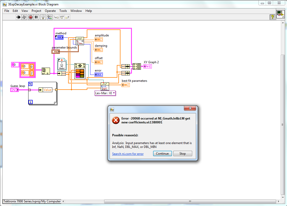
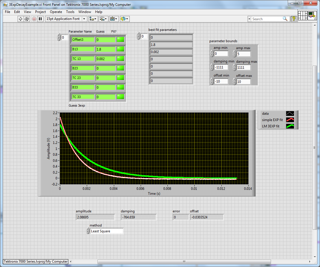
• Non-linear curve Fit error 20068?

  Trying to do a simple 3-exponential decay curve nonlinear.  I have a copy of this work in the other screws, but it doesn't seem to work in this VI.  I use "Scalablemultiexponentialdecay" of Altenbach as a VI/template model.  Data that I'm trying to adapt are a series simple decomposition RC, yes I realize that should not have 3 exponential components, it's just the model data.  I am able to adapt with the Fit exponential function built in to the Math palette, but which only works if the input bounds parameter is wired and with rational constraints.  However, I get an error on the adjustment of the non-linear curve that I understand not (photo attached) indicating that an INF or NaN is done in the settings.  I don't see where this is going...

  Any questions or help is appreciated.

  

  

  I thought so, only 0 s for the 2nd two exponentials.  But, if I replace all the guess seededes with the same as the simple exponential Installer, it converges without error.   I guess I didn't know it was that sensitive.  Thank you.

• coefficients variables semi in a non-linear curve fit

  Hi all

  I use a curved Lev - Mar not linear adjustment vi to fit a custom to my data function. The function is a set of Gaussian functions and an offset. I mean to constrain the width of one or more of the Gaussian curves in the function. I can do this by changing the values in the equation in the model description in the block diagram, but how to do this easily through the front?

  These width values will not be floated in the adjustment.

  Thank you!

  Unfortunately, the limited version was added in LabVIEW 8.5.  You could use the 'data' variant to pass the value of the stress sigma model and adjust the location and amplitude values. This means that your entry of Lev - Mar estimate does not include the values of sigma.  The value of sigma fixed wire entry "data".  Then depending on your model take data entry (type variant), cast to a value double precision and insert into the locations in your model formula.

  -Jim

• Non-linear curve fit the model of reference file

  Hello.

  I use the VI of the non-linear curve adjustment in order to adapt the data. The reference to the fitting VI model I use is included in the attachment. You can see that I have a few constant wireline, like 4, 2500 and 1. I want to do this constant variables I'll change before each curve corresponds, because actually in my problem this variables I know before the adjustment and they are constantly changing, and for the moment this made VI just to test.

  The problem I have is that I can't enter the values of this variable to my main VI, where I also call the VI was nonlinear. The scheme of connection of refernce VI made must be changed in order to be recognized by the VI was nonlinear. I tried to use a table to transfer variables, but if I use one, it recognizes the variables as parameters of editing and he's trying to install as well in the adjustment process, and it gives me erroneous results.

  Any ideas how I can add the values of variables?

  Thank you very much.

  Kind regards

  Nikola comedy

  To provide additional data randomly in VI of model, you must use the entrance of 'data' (it is a variant and so can contain anything you want!). Just create any type of data you want (generally a cluster if there are several values of different data types) that contains all the values, convert them to a Variant in the main VI and the variant of wire to crimp her. In the model, you convert the variant return to data, to the constant help of cluster, such as defined in the main as VI 'type' (simply right click cluster in the main VI... wire Create constant... move the constant in VI of model). Now, to unbundle the different values and use them anywhere inside your model.

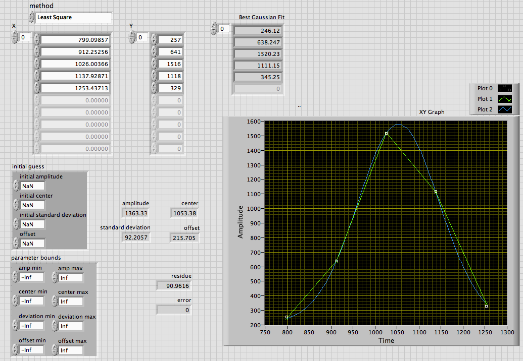
• Fit Gaussian Peak and non-linear curve Fit on small data differ from the PEAK of origin made

  Hi all

  I'm developing a program in which I have to adjust the curve of Gauss on only 4 or 5 data points. When I use the Gaussian Ridge Fit or adjustment of the curve non-linear, it connects linearly all the points so that other editing software like origin's curve fitting of Gauss on the same set of data that I have attached two images is LabVIEW with Fit Gaussian of Peak and nonlinear adjustment and other is original.

  The data are

  X                       Y

  799.09857 257
  912.25256 641

  1026.00366 1516
  1137.92871 1118
  1253.43713 329

  Interesting.

  The initial default values assume all are NaN, which causes the LV calculate conjecture.  The default values for the parameter Bounds +/-Inf with the exception of the offset that are both zero. This, of course, forces the output zero offset.  It seems a strange fault, but they may have a good reason for it.

  Change the limits of compensation to something else translates the output being offset ~ 215 and the Center moves to ~ 1053.  These correspond the original result to 5 significant digits.

  Lynn

  

• Curve adjustment not linear function

  Hello everyone:

  I'm a little new here and at the same time a new learner for labview. My need for laboratory to adjust the data which are not linear, so, I choose to use the model non-linear curve VI. But when I run the VI, the error is that:NI_Gmath.lvlib:LM formula function.vi:7290001 string, or other displayments of the error. I tried several times, but unfortunately didn't. The problem may be the expression of the function form. Moreover, the design of the VI is not mine, it's Forum OR. Any constructive suggestions will be welcome.

  The form:

  y = Y0 + (Nr * cos (A)) + *(x-W1)/((x-W1) a1 ^ 2 + L1 ^ 2) + a2 *(x-W2)/((x-W2) ^ 2 + L2 ^ 2)

  In fact, the form is very long, I just write some.

  
  

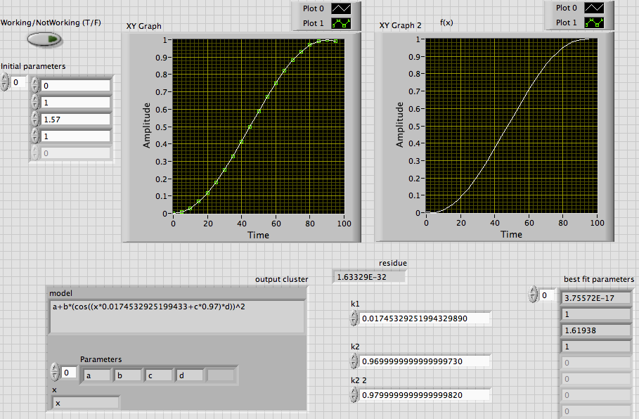
• Need help with the non-linear curve - fit

  Hello

  "I enclose you a VI that calls the function of nonlinear smoothing" Lev - Mar "with two slightly different formulas.

  On my machine (Win7, LV2011) adjustment is a straight line when bool example FP is set to FALSE.

  This is expected behavior?

  Is it possible to get a good fit, with the coefficient of 0.97 and _without_ increase in the number of points?

  Thanks in advance!

  I've just implemented the formula to the fitting VI.  I did not review the calculation you did for "raw" data

  Review: The first value of x is equal to zero. To get a phase shift of ~pi/2 a good first guess for c is 1.57.  With a value close to that, it gives a good fit for each choice of c.

  

  Lynn

• apply restrictions for the non-linear curve fit

  Hello Forum users,.

  I am currently working on a VI control which is supposed to create a specific model of pressure inside a hollow tube to provide a test environment for pressure sensors. The details are many and complicated, so let's say I am sure that my formula to calculate this profile according to the pressures inside the hollow rings around this tube will work.

  To find the correct pressure for each ring values, I've linked to a model VI containing this form to Lev. - Mar algorithm (the non-linear curve adjustment) and let it run.

  Technically, there is no problem and Lev - Mar find values to adjust the function for the values (not perfectly sure, but close enough).

  The problem is, however, that, since the device, once suitable values for the positioning and size of the rings are found, must be built, the simulated pressure rings perhaps intersect not between them. To apply this rule, I added a check to my VI of model and if the values passed to Lev - Mar breaking the rules, the VI model gives a matrix of zeros to follow him (I tried an empty array, but that only leads to error messages).

  This solution did not work. Lev - Mar seems to ignore these cases always looks for values that break my rules (and if I put these values through my model VI, I get a matrix of zeros, as expected, so the audit seems to work).

  Perhaps I misunderstood the algorithm of Lev - Mar and it does not actually check each possible defined coefficients of finds.

  Is it possible to adapt to any function of a set of values while keeping the predefined boundary conditions?

  Oh, before I forget:

  I use LabVIEW version 8.2 in the Institute, because the workshop systems is not installed 8.5 for some reason any.

  Thanks in advance

  Thaliur

  Hi Thaliur,

  Thanks for posting on our forums.

  I understand your request you expect the algorithm to ignore a case to all zeros in the table. However, it is not implemented like this.

  Good news is, its source code can be edited and you could save your own personalized version of the algorithm of screws it is to you that you just add a check for a matrix of zeros or simply pass another parameter which indicates only a case of "broken rules". Then you would not have to continue the calculation.

  If I misunderstood your question, please clarify this. You can also post a code for further explanation, if you wish.

  Good luck with the project!

  Peter

• Non-linear function Lev - Mar - output gradient functions reference table?

  Hello

  I have the whole 8.6 developer and am relatively new to labview.  First time posting, but these tips already have a lot of my problems solved.  Thank you!  My luck ran out however...

  I had worked on a recursive function to fit a set of nonlinear data, when I stumbled upon the function of lev - mar.  What a great discovery... it works very well.  However, I tried to determine the criteria for the named 'f '(X,a)' reference to the static VI which contains the lev - Mar function to fit the output.  The function performs fine without her that it will calculate the slopes in itself if the gradient table is empty, but it takes a little more time and I'm trying to speed up a bit.

  The example 'Fit Gauss surface with offset.vi' is the only example I could find where the output of f'(X,a) of the reference to the function VI is populated, but I'm a little rusty with my calculations and has failed to reverse engineer exactly what should be the values that they had classes in this table.

  I would like to be able to complete the table of f'(X,a) with the data of a 2d versus 3d surface curve in the example 'Fit Gauss surface with offset.vi.  Is attached a screenshot of the example showing the output in the example of f. '(X,a).

  Thank you very much!

  -Bill

  If you do not provide the analytical partial derivatives, LabVIEW will use automatically digital derived partial. You can watch the labview code in detail to see how it does, just open the VI and search for "LM digital gradient.vi.

  I don't know what, "recursive function" in this context, but they have an analytic expression for the partial derivatives?

  Even if the analysis of the partial derivatives are not possible, it may be an advantage to making your own derived partial inside the model. It seems to be much faster.

  You'd basically is to calculate the function several times, each time with one of the parameters that is incremented by a small delta and subtract function calculated with the current settings Plains each and divide the result by the delta. Do everything in a table 2D for the output of f'(X,a).

  The image shows one way to do this inside the model. The black square is a model where you replace you own function (f(x,a)).

  

  Let me know if you have any questions.

• The non-linear curve fit lev mar problem

  Hi, I have a set of 10000 readings recorded every second. My goal to draw these vs time readings (1-10000 s) in logarithmic scale and adjust the exponential curve that results with my model equation: a1 * exp (t * b1) + a2 * exp (t * b2) + a3 * exp (t * b3) + a4 * exp (t * b4) and get the values of the coefficients (a1 to a4, b1 - b4). I changed the non-linear adjustment of lev - mar.vi according to my model. However, I ran into a problem.  I get the following: error-20041 occurred at LM.vi:5 to get on the curve of the NI_Gmath.lvlib:Nonlinear Possible reason (s): the system of equations can be solved because the input matrix is singular. I can't work on why I get this error. I enclose 3 files: the data file (values of Y), X = 1-10000; coating not get my model and vi vi.

  I'm using Labview 8

  I would appreciate your help and suggestions! Thank you very much in advance. ANU

  Hello

  @Jim-thank you very much... ur modified vi helped a lot... but a strange thing on the adjustment is that it depends a lot on the estimation of the coefficients... my model should have values of 'a' coeffs in the order of 10 ^-7 and 'b' should be higher around 10 ^-1. The initial proposal is amended the best coefficients made vary accordingly.

  I don't really know if this can b fixed... I enclose my vi.

  VI: - non - linear adjustment model, exponential branch.

  data - pol.txt

  I appreciate you all!

• Isoquant linear function

  Hi all

  Problem of basic but I would like some advice:

  I have a series of points (which is an approximation of a more complex curve).  I want to get linear lines between each of the points.

  The end result should be a VI I can feed a value x in and return a value y for the entire range covered by the series of linear lines (equations).

  The best way to go about this?

  

  Thank you

  Battler.

  G ' Day David,.

  Thanks for your help.

  I think I have solved with this:

  

  No point reinventing the wheel!  NOR did the job for us.

  I think that we can get our x and are involved.  I probably communicate better.

  I want to be able to enter a value for x (col (0)) and come up with a value of y (col (1)).

  For example. If I put x = 750 it returns y = 75, which seems fair to me...

  Thank you for helping me find these useful screws

• PIECEWISE LINEAR VOLTAGE Source BUG

  I want to source PWL allows to analyze signals from my digital oscilloscope.

  File MEANDR.txt contains 5000 points of voltage (mV) in the time domain.

  (1) if I'm going to use this file with the option 'Use data directly from files' there will be no signals at the output of the source.

  (2) if I go use the option "enter data points in the table---> Initialize the file" and press the button "Run the Simulation" Multisim breaks down... but it starts working properly if I'll burn the original file of 5000 points to 2000-300 points. (File MEANDR_MODIFIED.txt)

  You can fix this bugs?

  Thank you!

  Hi, ZG,.

  Your data will give Multisim a problem because of the format, Multisim expects the tension and the time of two columns.  On the column of time data range from 1 to 5000 so Multisim will have to simulate for more than an hour and in the world of simulation that is an eternity.  I changed the data so that Multisim simulates only up to 5 sec.  Your column of tension is supposed to be in mV on each line, you will need to place a mili at the end otherwise Multisim going out KV. Using Word and Excel, I changed your data to something that Multisim may include and the file is associated.

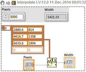
• No linearity between the pixels and width of linear scan

  Hello

  I develop a gauge width based on a linear scan camera.

  The gauge is to measure the surface of a strip steel moving at 200 m/s.

  I found a non linearity between the relationship of pixels and the actual width:

  1904 mm X 6635, 6pixels

  1308 mm X 4616, 7pixels

  814 X 2880 mm, 6pixels

  I tried the distances of work between 2600 to 2800mm.

  The field of vision is 2200mm.

  The focal length is 35 mm.

  The size of the CCD is 28.67 mm (3.5um X 8192pixels - Basler raL8192 - 12 gm).

  Someone has already faced this problem?

  Thank you

  Alexander.

  There are many ways to do it, as the adjustment of an equation in your data that you can then use, but if you want to be fast (and if you use a very quick line scan camera, so I assume you are), I think the fastest way is to use a table like this:

  

  This simply assumes that the relationship is piecewise linear, i.e. linear between point each of your measured data (and that you have already provided three).  Keep filling in the Bay of cluster with paired values (pixels, width), ensuring that the values are in a strictly ascending and 1 d interpolating function Array used here does all the work and seems to be very fast too.  You only need enough points in the table to make your quite precise interpolation for your needs.

  There are certainly ways to do it though, so someone else might have a better suggestion.