value of single cell

Similar Questions

• How to display row values in a single cell, separated by commas?

  Hello
  I have a table of opportunity and at every opportunity, there are several values from the provider in the table Vendor, i.e. relations ship between the table of the opportunity and the seller, the table is 1:m.
  In the reports, I want to show all providers for the occasion in a single cell, separated by commas.
  For example Oppty1 has Ven1, Ven1, Fri 3 in table.so of sellers in reports that it should show as
  
  ________________________
  Opportunity | Seller |
  ________________________
  Oppty1 | VEN1 Ven2, Ve3 |
  ________________________|
  
  Please help me with the approach of implementation, I have to take for it.
  
  Thank you
  Anamika

  Visit this link,

  Re: Display of the horizontal values

  Thank you
  Vino

• Derivative of a cell based on the value of another cell's true/false

  Hello

  I try to create a list of digital control and would have put cells highlight according to a corresponding value in another cell.

  For example, I would like cell D2 to white if the cell H2 is FALSE, or if the values of H2 is TRUE, I would D2 to be green. I want this for about 20 lines.

  Any suggestions?

  Hi JCR.

  Conditional highlighting rules depend on comparing the value contained in the cell to be highlighted (D2) with a second value. The second value may be fixed (recorded in the rule) or may be contained in a cell of the second.

  In your scenario, the highlight would be independent of the value in D2.

  There are two ways to accomplish what you want using conditional highlighting, highlighting a third cell whose value depends on the value in H2 and whose pointing out will be seen as highlighting of the D2, OR by providing a third cell whose value can match or does not match the value in D2 , the value of H2.

  Since you want to highlight only a single cell, and not a group of cells, the second method is probably more simple here.

  

  Each cell in the column I contains the following formula, entered in I2, and filled then down on the rest of the column:

  I2: = IF (H, D, "xxx")

  English: If the cell in this row of column H is set to TRUE (enabled), copy the value in this row of column D to this cell. If not, put "xxx" in this cell.

  'xxx' can be any value that will be ever present in the cells in column D.

  The below table conditional formatting rule is placed in cells D2 - D10. The cell reference is to the cell "this rank" in column I and is different for each cell.

  Kind regards

  Barry

• Can LabVIEW VIs database connectivity write an array to a single cell?

  Hello world

  I wonder if DB tools insert data VI is able to accept a table as its input. It's a bit difficult to say because all connect you to the input of this VI is voluntarily accepted by the terminal, data type variant so no glaring broken threads occur when associate you a table.

  What I'm trying to do, it is write a table 2D of doubles in a single cell in a table. The table is large 3 x 1000 elements. I confess to being completely new to databases and such an effort may or may not look ridiculous in the database world. If someone wants to talk about why I'm trying that I'll gladly go through my reasoning - just enough to say that I'm not totally crazy.

  When I try to write the table to a single cell, an error as seen in the attached screenshot. All my other functions database, working with scalar values of many different types of data, all work very well.

  I have attached the problematic code. It tries to write these tables 8 to 8 individual columns, all in the same line. I'm just using the method "automatic" for now.

  Extra tid bit of information:
  OpenSQL database. Connection via ODBC 5.2 64 bit, user DSN.

  LabVIEW 2012 not SP1. Windows 7 64-bit.

  Thank you all!
  Rhys.

  Convert the table to a spreadsheet string and store it like that.

  

• Problem of format of letters in single cells

  Hi, question maybe an IE6 and not DW8...
  I built a calendar using tables with individual cells. The numerical values are sitting nicely in their cell, but the header cells (M T W T F S S) even if OK in DW8 extend downwards by a single cell in IE6. I guess that's a white character and would like to lose! Any ideas please on how to solve this problem would be appreciated. I am not not familiar with CSS and hope that there is an alternative that I can use. Regards, Barry

  November 28, 2006 to macromedia.dreamweaver, barryc433 wrote:

  > I built a calendar using tables with individual cells. The
  > numeric values to sit
  > nicely in their cell, but the header cells (M T W T F S S)
  > even if OK in DW8 extend downwards by a single cell in IE6.
  > I guess that's a white character and would like to lose! Any
  > thoughts please on how to solve this problem would be appreciated. I have
  > am not not familiar with CSS and I hope that there is a
  > alternative I can use. Regards, Barry

  > You can see if you check out the following -.
  > http://www.paradisecityrentals.com/calendar.htm

  Try to get rid of the

  tags in headers.

  --
  Joe Makowiec
  http://Makowiec.NET/
  E-mail: http://makowiec.net/email.php

• How can I use highlighting conditional to assign a cell using the value of another cell

  I would use conditional highlighting on a cell based on the value of another cell.

  For example:

  If K2 is 1, then I would than A4 Green

  Any suggestions?

  Hi louis,.

  This approach is to add a cell to compare your target for:

  

  Highlight the rule in this case:

  

  Quinn

• Paste multiple lines of text in a single cell in a table

  Hi all

  I lost it by train for formatting columns and thought it would be easier to put the data in a table.

  I tried selecting my 5 lines (name and address) and paste it into a single cell of a table, but it keeps splitting up to more than 5 cells.  Is any way to replace it?

  Thank you

  Hey Shorty,

  Select the 5 lines of text and copy (or cut).

  In a table cell, click twice to place the cursor in the cell (the cursor is now in the text layer of the cell).

  Dough.

  

  Kind regards

  Ian.

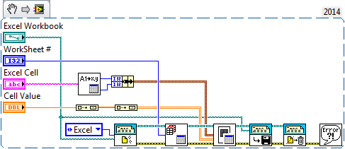
• Replace different values in different cells

  Hello

  I'm new to LabVIEW and work with a tool that retrieves its settings in an Excel file. I need to change these settings in Excel using LabVIEW. The Excel file is formatted as .xls (97-2003 version). The PC has Microsoft Office installed 2013.

  I'm using LabVIEW 2014 (64-bit).

  Task:
  I want to change the values in 3 different cells in an Excel worksheet and save the workbook (not save as).
  The main vi is saved in the library in the zip file, it is called 'change the 3 values in excel.vi '.
  The excel file is fixed separately.
  I don't think that it matters where these cells are in the Excel worksheet, Excel memory seems to remember the selection of cells in all cells but replaces the value with the last mentioned in the last under vi.

  Problem:
  (1) any change of cells to the same value that I set in the third sub vi.
  (2) Excel wonder SaveAs and does save not only on the existing file.
  (3) the Excel application is not closed, but I can't understand why.

  Please advice. Help on all these issues is highly appreciated.

  Thank you!

  Here is how I could do this.  I would use the Report Generation Toolkit (which is included in LabVIEW 2014).  This example is a simplified version of your task-you are given the name of an Excel workbook to change, the index of the worksheet to be used, the cell address Excel (in format Excel, for example, A1, for example) and the value of the cell that you want to insert here.

  

  The first function is the new report, which is a slight misnomer, as we use it as 'Report to replace' wiring on behalf of the State existing and specifying that we hear an Excel report (it opens Excel - if you don't want the workbook to be visible, open it reduced).  We then call get Excel spreadsheet (which is not necessary if we use the first worksheet...).  We use Excel table easy to put the value of the cell in the Excel cell chosedn.  To do this, we first use Excel Excel get a location to convert, say, B3, line/column indexes (B3 = 1, 2) and this group in a Cluster.  We also need to convert the value of the cell in a table 2D what we do by passing through two functions of table build.  Then save us report to the file using the original Excel workbook path and finally alienate us report goes out Excel.

  If you had multiple cells that you want to update, I would like to consolidate Excel cell and cell value in a cluster, build an array of clusters, then put the Excel easy table function in a loop, and do the updates one at a time.

  It should work very quickly - the whole process should take a fraction of a second.

  Bob Schor

• How to read a value from a cell in a row

  Hello;

  I need the name of a function that is able to read a value from a cell in a row. the line contains multiple values.

  If you can post for me, I grow

  
  

• Using excel, if I remove a value in a cell and you decide then he should not have been deleted, how I get it back?

  Using excel, if I remove a value in a cell and you decide then he should not have been deleted, how I get it back?

  Once you have removed the cell values and you have not saved the document again that you can always undo changes.

  Keyboard shortcut for undo is Ctrl + Z.

  MD MOEEN AJAZ KHAN - MCP, N +, A +.

• The value of the cell in column

  Hello
  
  We report with a number of columns and columns of cells have value with a lot of characters (more than 100). We want to adjust the value of the cell in this column for example 20 characters and all characters of the value of the cell in column value of title HTML TD as "flag". Something like this:
  
  < code >
  "< td #ALIGNMENT headers # =" "#COLUMN_HEADER_NAME #" title = "#FULL_COLUMN_VALUE #" class = "data" > #TRIMED_COLUMN_VALUE # < table >
  < code >
  
  We can do as a model? You have an idea?
  
  I have an idea that uses JavaScript and the value of the total column in the hidden column, but I thing that there could be a better way to do this :-)
  
  Regarding.
  
  David
  
  Published by: user4893970 on November 23, 2010 16:11

  While I don't think that there is a way to do it with a normal report

  If it's a standard and not interactive report, then it can be done using the column Expression of HTML:

  #TRIMMED_COLUMN_VALUE#
  

• Copy the value of a cell in another tab.

  Hello

  First of all, I'm french. I hope you could understand my poor English.

  I have a got a form with a tab where you can sup or ad raws.

  I gat a second tab.

  I would like to copy the value of the cell (textfield) in a cell in the second tab.

  I try ' this.rawValue = evolution.forobj.tab1.r1.txt1.rawValue; ' event, but it does not change.

  Thanks for your help.

  Nath

  Hi Nath,

  This should work in case the object in tab2 calculate:

  this.rawValue = evolution.forobj.tab1.r1.txt1.rawValue;
  

  The language must be set to Javascript.

  There is another way to approach this problem without script. So, if you can not get this to work, come back.

  Niall

  Ensure the dynamics

• Return all column names of the cells that match a value in a single cell

  

  I want to be able to scan all the cells in column 1 in column 3 (there could be several) which belong to the same line and check if they all have a value y (X). If they have no value, I want all columns to display all the names of the matching columns as follows: "column 1, column 2" for Elemento.

  This can be a good start:

  

  B2 = if (counta (C2) > 0, C$ 1, "" ") & IF (COUNTA (D2) > 0', ' & D$ 1," ") & IF (COUNTA (E2) > 0', ' & E$ 1," "") & IF (COUNTA (F2) > 0', '& F$ 1,' ')

  It's shorthand dethrone select cell C2, then type (or copy and paste it here) the formula:

  = IF (counta (C2) > 0, C$ 1, "" ") & IF (COUNTA (D2) > 0', ' & D$ 1," ") & IF (COUNTA (E2) > 0', ' & E$ 1," "") & IF (COUNTA (F2) > 0', '& F$ 1,' ')

  Select cell B2, copy

  Select the cells B2 the bottom of column D, dough

  To add additional columns, you copy the atomic unit:

  & IF (COUNTA (D2) > 0', '& D$ 1,' ')

  and update D2 with the new column and D$ 1 with the new column.

  then... If you add a new column (G, for example) that you want to change it:

  and IF (COUNTA (D2) > 0', '&D$1,' ')

  TO

  and IF (COUNTA (G2) > 0', "&G$1," ")

  and the updated formula would be:

  = IF (counta (C2) > 0, C$ 1, "" ") & IF (COUNTA (D2) > 0', ' & D$ 1," ") & IF (COUNTA (E2) > 0', ' & E$ 1," "") & IF (COUNTA (F2) > 0', ' & F$ 1,"") & IF (COUNTA (G2) > 0', '& G$ 1,' ')

  fill down like before

• How to format a single cell based on the value in another cell?

  IM using JDEV 11.1.2.4 and had the following use cases.

  based on a threshold value in a column of my line, I want to show a different value in the color red.

  How to get there?

  Hello

  This could be a possible solution using inlineStyle and a simple logic of EL

  inlineStyle = ' #{rank. " TRESHOLD > 10? "{" color: #990000 ': "color: #000000 '} '.

  ID = "ot1" / >

  Marc

• I need to do at several levels of values in a cell

  I need a formula to give me several different levels on a cell.  More precisely;

  First % of $100,000 = 2,175

  % Of $400,000 = 1,305 following

  Next $2,000,000 = 8.7 percent

  Next $2 500 000 = 6.55 percent

  Next $2 500 000 = 6.1 percent

  More than $7,500,000 = 5.65 percent

  I have a formula in an old worksheet that works, but my values have changed, and I can't figure out exactly why it works.  I'm an amateur trying to look professional.  AMOUNT (0.25, 0.75% × G5 %×MIN(G5,2000000),0.5%×MIN(G5,500000),1%×MIN(G5,100000)))

  Hi stephanie,.

  Use a lookup table. This makes it easy to modify the thresholds and rates without having to rewrite the formula.

  Here's an example, using the rates and thresholds in your message.

  

  INT is the first two columns of search table.the are given seizure - threshold amounts in column A and the interest rate from thea threshold in column B.

  Column C contains the following formula, which is used to calculate the interest charged at each threshold.

  C2: entered value - 0 (zero)

  C3: = B2 + C2 × (A3−A2)

  Fill to last line requiring this calculation (line 7 in the example).

  MAIN is the table on which the interest due is calculated.  The amounts are recorded in column A, all other values in the table are calculated. Calculation has been spread over four columns to display each step separately. the whole calculation can be done in a single column, using the formula below.

  All formulas are entered in row 2, and then fulfilled down to the number of lines needed for the calculation of the amounts of the different loans.

  B2: = LOOKUP($A,INT::$A,INT::B)

  The interest rate on the amount greater than the amount of threshold spent last search.

  C2: IS EQUAL TO LOOKUP($A,INT::$A,INT::C)

  Research the amount of interest on a loan to this increased threshold amount.

  D2: = B × (($A, INT::$A) A−LOOKUP)

  Look up to the last threshold amount spent, which subtracts the amount of the outstanding loan and multiply the result by the interest rate in column B.

  E2: = C + D

  Calculates the changes of total interest by adding the due interest on the amounts until the last threshold and the interest due on the amount exceeding this threshold.

  The four formulas can be combined as follows, to return the same result:

  F2: = LOOKUP($A,INT::$A,INT::C) + (A−LOOKUP($A,INT::$A)) × LOOKUP($A,INT::$A,INT::B)

  Kind regards

  Barry